Building high-resolution transport matrices from ACCESS-OM2 outputs

TLDR: I want to build high-resolution transport matrices from ACCESS-OM2 outputs and use them to study ocean ventilation. I’ve had a couple back and forth emails with @aekiss about the outputs I need, and we thought it would be best to continue here so that others can chime in (to help but also maybe benefit) from the discussion.


To build Transport Matrices (TMs) from ACCESS-OM2 outputs, I need 3D mass transport in x/y directions, mixed-layer depths, and cell geometries (vertices, volume, area, and thickness). I can build the cell volumes from area and thickness, and I can get the cell vertices from the supergrid files separately. For the rest, I need these variables:

  • tx_trans and ty_trans(resolved mass transport)
  • tx_trans_gm and ty_trans_gm(GM mass transport; not for 0.01°),
  • mld(mixed-layer depths)
  • area_t (tracer cell horizontal area)
  • dzt or dht (tracer cell thickness; quick question in passing, does dzt = dht?)
  • and optionally tx_trans_submesoand ty_trans_submeso(sub-meso scale mass transport; “optionally” because these are small… right?)

In case it is useful to others (or if you find something wrong with it), I’m sharing the code I used to query the ACCESS-NRI catalog just below. It filters for all the ACCESS-OM2 runs that include the variables I listed above.

import intake
catalog = intake.cat.access_nri

# comment/uncomment to filter variables
variable=[
    "tx_trans", "ty_trans",
    # "tx_trans_gm", "ty_trans_gm",
    # "tx_trans_submeso", "ty_trans_submeso",
    "mld", 
    "area_t",
    # "dzt",
    "dht",
]

variables_set = set(variable)

query = dict(model="ACCESS-OM2.*", variable=variable)

df = catalog.search(**query).df
df = df.groupby('name', as_index=False)['variable'].sum()
df['variable'] = df['variable'].apply(lambda x: set(x))

filtered_df = df[df['variable'].apply(lambda x: variables_set.issubset(x))]
filtered_df.name

Here are all the experiments with everything I need (including GM for 0.25° and 1°, but ignoring whether submeso is included or not):

01deg_jra55_ryf_Control
01deg_jra55_ryf_ENFull
01deg_jra55_ryf_LNFull
01deg_jra55v13_ryf9091
01deg_jra55v13_ryf9091_easterlies_down10
01deg_jra55v13_ryf9091_easterlies_up10
01deg_jra55v13_ryf9091_easterlies_up10_meridional
01deg_jra55v13_ryf9091_easterlies_up10_zonal
01deg_jra55v13_ryf9091_qian_wthmp
01deg_jra55v13_ryf9091_qian_wthp
01deg_jra55v13_ryf9091_weddell_down2
01deg_jra55v13_ryf9091_weddell_up1
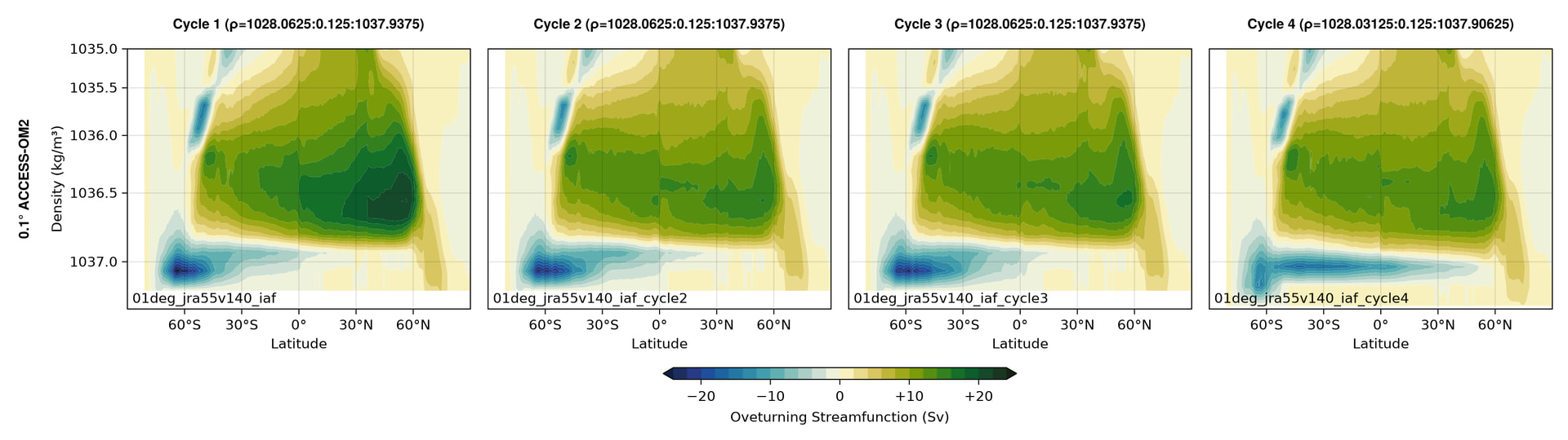
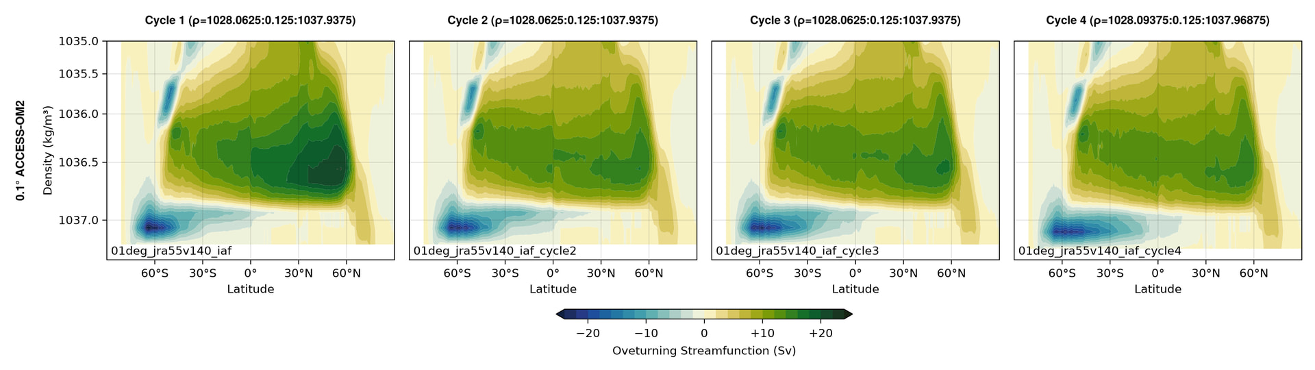
01deg_jra55v140_iaf
01deg_jra55v140_iaf_cycle2
01deg_jra55v140_iaf_cycle3
01deg_jra55v140_iaf_cycle4
01deg_jra55v140_iaf_cycle4_jra55v150_extension
01deg_jra55v150_iaf_cycle1
025deg_jra55_iaf_omip2_cycle1
025deg_jra55_iaf_omip2_cycle2
025deg_jra55_iaf_omip2_cycle3
025deg_jra55_iaf_omip2_cycle4
025deg_jra55_iaf_omip2_cycle5
025deg_jra55_iaf_omip2_cycle6
1deg_jra55_iaf_omip2_cycle1
1deg_jra55_iaf_omip2_cycle2
1deg_jra55_iaf_omip2_cycle3
1deg_jra55_iaf_omip2_cycle4
1deg_jra55_iaf_omip2_cycle5
1deg_jra55_iaf_omip2_cycle6
1deg_jra55_iaf_omip2spunup_cycle1
1deg_jra55_iaf_omip2spunup_cycle2
1deg_jra55_iaf_omip2spunup_cycle3
1deg_jra55_iaf_omip2spunup_cycle34
1deg_jra55_iaf_omip2spunup_cycle35
1deg_jra55_iaf_omip2spunup_cycle36
1deg_jra55_iaf_omip2spunup_cycle37
1deg_jra55_iaf_omip2spunup_cycle38
1deg_jra55_iaf_omip2spunup_cycle39
1deg_jra55_iaf_omip2spunup_cycle4
1deg_jra55_iaf_omip2spunup_cycle5
1deg_jra55_iaf_omip2spunup_cycle6
1deg_jra55_ryf9091_gadi

Unless I forgot something or made a mistake, any other ACCESS-OM2 run is missing one of the variables I need. My issue is that the only 0.25° runs with GM are the 025deg_jra55_iaf_omip2_cycle* ones, and while it’s great to have the corresponding 1° runs (1deg_jra55_iaf_omip2_cycle*), as far as I know there are no corresponding OMIP2 0.1° runs… Is that right? Is there a consistent set of (1° + 0.25° + 0.1°) runs with the outputs I need that I may have missed? Is the Intake catalog up to date or should I go digging for these outputs “by hand”?

Also happy to discuss any other aspect of this project :smiley: just let me know!

1 Like

@Benoit thanks for sharing your plans up on the forum (so sorry, I still haven’t replied to your email on this – it’s on my todolist!)

But regarding OM2 GM availability, if you haven’t seen it, this discussion might be a little helpful?

On these points:

Is there a consistent set of (1° + 0.25° + 0.1°) runs with the outputs I need that I may have missed?

I think @aekiss @AndyHoggANU @rmholmes @adele-morrison might know?

Is the Intake catalog up to date or should I go digging for these outputs “by hand”?

@dougiesquire and @CharlesTurner might have some thoughts on this…?

Hi @Benoit,

Yes. dht is just the CMIP name. Same variable.

As far as I know 01deg_jra55v140_iaf_cycle* is consistent with the 025deg_jra55_iaf_omip2_cycle* and 1deg_jra55_iaf_omip2_cycle* simulations. They all use JRA55-do v1.4 forcing (I just checked the github repos for this, listed at ACCESS-OM2 Control Experiments ). The 1/4 and 1-degree runs were the ones submitted to OMIP-2. There will obviously be differences w.r.t. numerics, parameterizations etc., but you’re expecting that. What other measures of consistency are you looking for?

1 Like

Thank you @rmholmes! This is very useful :slight_smile:
I think that’s good enough for me for consistency…

1 Like

We updated the catalog on Thursday/Friday last week, so the catalog should be up to date.

1 Like

Hi @Benoit, as @rmholmes said, the ACCESS-OM2 Control Experiments are our most consistent configurations spanning the 3 resolutions.
01deg_jra55v140_iaf* seem to have the variables you need, other than tx_trans_submeso - see
Data available: 0.1° 1958-2018 ACCESS-OM2 IAF runs (plus extension to 2023) – COSIMA

1 Like

I was going to suggest passing require_all=True to catalog.search() to achieve this. But this produces unexpected results for conda/analysis3 > 25.07.

With conda/analysis3-25.07, I think the following will give the list you are after:

import intake
catalog = intake.cat.access_nri

variable=[
    "tx_trans", "ty_trans",
    # "tx_trans_gm", "ty_trans_gm",
    # "tx_trans_submeso", "ty_trans_submeso",
    "mld", 
    "area_t",
    "^d[hz]t$",
]

catalog.search(
    model="ACCESS-OM2.*",
    variable=variable,
    require_all=True
).unique()["name"]

I’ll open an issue about the unexpected behaviour for conda/analysis3 > 25.07 so that we can get this fixed up. UPDATE: issue opened here.

1 Like

Very neat, thanks!

Did something change between cycles 3 and 4 for the OM2-01 IAF runs?

I noticed a substantial “jump” in the deep circulation between 01deg_jra55v140_iaf_cycle3 and 01deg_jra55v140_iaf_cycle4 and I’d like to understand what drove this jump.

If you look at the MOC streamfunctions averaged over each cycle, you can see that the bottom cell extends much further to the north in cycle 4 (4th panel in image below):

Comparing the time series of AABW transport at 40°S (taken as minus the minimum of the streamfunction at 40°S below 1036 kg m⁻³; top panel in image below) shows some change between cycles but nothing suspicious. However, at 20°N (bottom panel), the difference is striking:

Could this is related to the reproducibility issues / bugs about these runs discussed on the Hive and on GitHub?

cc @aekiss @LaurieM

Interesting! I don’t think anything changed, but @aekiss will know. The disconnect between the end of the 3rd cycle and start of the 4th cycle in that last plot seems concerning.

Sorry for my slow reply, and thanks for asking @Benoit - I hadn’t noticed that before.

It also looks to me like the unsmoothed timeseries (translucent lines) are discontinuous between most cycles at both latitudes.

Here are all the differences between the last run of cycle 3 and the first run of cycle 4 (using git hashes obtained from the run summaries for cycle 3 and cycle 4).

Cycle 4 uses BGC in both MOM and CICE, with different executables for all 3 components, so it would be a concern if that has altered the physical model.

On the other hand, cycle 4 also doubles layer_nk from 80 to 160, so maybe increased resolution in density space could explain your results?

chio and snowpatch are apparently also changed (not sure if the latter differs from default). [edit: these aren’t actually changed - see below]

I don’t think it’s related to the non-reproducibility issue you linked to, as this happens during a run, not between restarts.

1 Like

Here are all the MOM5, CICE5 and libaccessom2/YAML code changes between cycle 3 and cycle 4.

The CICE parameter chio=0.004 was ignored in cycle 3, and defaulted to 0.006, so in cycle 4 we fixed this bug and set chio=0.006 explicitly. So in practice we had chio=0.006 in all cycles.

snowpatch=0.02 is the default, so that’s also unchanged between cycle 3 and 4.

1 Like

With these cycle 4 parameters we have data on density 1038kg/m3 and above, at increments of 10/160=0.0625 kg/m3. The density resolution is twice as coarse in cycle 3 (10/80=0.125 kg/m3), which seems like it could be too coarse to capture the narrow density range in which you find the streamfunction maximum in cycle 4 at 20°S. So this is plausibly just an issue with diagnostic resolution, not the model state itself.

1 Like

Thanks a lot for the investigative work @aekiss!

Would it help to plot the overturning in depth space (i.e., from ty_trans) instead of density space? (Actually I might as well plot it since that’s what I use to build the matrices anyway. Will post plots here when they’re done.)

Yes - if my guess is correct, the overturning in depth space won’t show much change between cycles 3 and 4.

A more direct check would be to plot cycle 4 in density space but with every second density level removed so the levels are the same as in cycle 3.

1 Like