Thank you so much. Now I put the test data on /scratch/public/rh1363/
Anyone can use the follow code to test it without any change.
##load
import numpy as np
import xarray as xr
import pandas as pd
import os
from xmitgcm import open_mdsdataset
import xgcm
#ecco_v4_py
import sys
from os.path import join,expanduser
user_ECCO_dir = ('/scratch/public/rh1363/ECCOv4-py/')
sys.path.append(join(user_ECCO_dir,'ECCOv4-py'))
import ecco_v4_py as ecco
import warnings
warnings.simplefilter('ignore')
os.environ['PYTHONWARNOINGS'] = 'ignore'
#for plot
import matplotlib.pyplot as plt
import cartopy.crs as ccrs
import cartopy.feature as cfeature
import cartopy.mpl.ticker as cticker
from cartopy.util import add_cyclic_point
##load data
data_uv = xr.open_dataset('/scratch/public/rh1363/uv_test.nc')
data_uv.attrs=[]
data_uv.load()
# define the connectivity between faces
face_connections = {'face':
{0: {'X': ((12, 'Y', False), (3, 'X', False)),
'Y': (None, (1, 'Y', False))},
1: {'X': ((11, 'Y', False), (4, 'X', False)),
'Y': ((0, 'Y', False), (2, 'Y', False))},
2: {'X': ((10, 'Y', False), (5, 'X', False)),
'Y': ((1, 'Y', False), (6, 'X', False))},
3: {'X': ((0, 'X', False), (9, 'Y', False)),
'Y': (None, (4, 'Y', False))},
4: {'X': ((1, 'X', False), (8, 'Y', False)),
'Y': ((3, 'Y', False), (5, 'Y', False))},
5: {'X': ((2, 'X', False), (7, 'Y', False)),
'Y': ((4, 'Y', False), (6, 'Y', False))},
6: {'X': ((2, 'Y', False), (7, 'X', False)),
'Y': ((5, 'Y', False), (10, 'X', False))},
7: {'X': ((6, 'X', False), (8, 'X', False)),
'Y': ((5, 'X', False), (10, 'Y', False))},
8: {'X': ((7, 'X', False), (9, 'X', False)),
'Y': ((4, 'X', False), (11, 'Y', False))},
9: {'X': ((8, 'X', False), None),
'Y': ((3, 'X', False), (12, 'Y', False))},
10: {'X': ((6, 'Y', False), (11, 'X', False)),
'Y': ((7, 'Y', False), (2, 'X', False))},
11: {'X': ((10, 'X', False), (12, 'X', False)),
'Y': ((8, 'Y', False), (1, 'X', False))},
12: {'X': ((11, 'X', False), None),
'Y': ((9, 'Y', False), (0, 'X', False))}}}
# create the grid object
grid_llc = xgcm.Grid(data_uv, periodic=False, face_connections=face_connections)
zeta = (-grid_llc.diff(data_uv.UVELMASS * data_uv.dxC, 'Y',boundary='fill',fill_value='NaN') +
grid_llc.diff(data_uv.VVELMASS * data_uv.dyC, 'X',boundary='fill',fill_value='NaN'))/data_uv.rAz
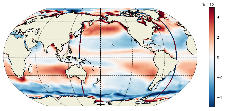
# plot the wrong result
plt.figure(figsize=(12,5), dpi= 90)
ecco.plot_proj_to_latlon_grid(data_uv.XG, data_uv.YG, \
zeta.isel(k=0), \
user_lon_0=180,\
projection_type='robin',\
plot_type = 'pcolormesh', \
dx=0.25,dy=0.25,show_colorbar=True,\
cmin=-1.e-6,cmax=1.e-6);
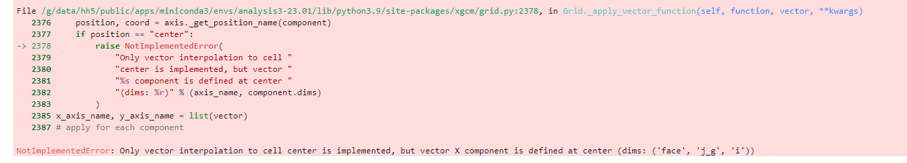
# the following do not work
zeta0=grid_llc.diff_2d_vector({'X': (data_uv.VVELMASS * data_uv.dyC), \
'Y': (data_uv.UVELMASS * data_uv.dxC)},\
boundary='fill')
zeta2 = (zeta0['X'] -zeta0['Y']) / (data_uv.rA)